3.3.4 사이킷런을 사용하여 로지스틱 회귀 모델 훈련
앞 절에서 아달린과 로지스틱 회귀의 개념적 차이를 설명하기 위해 코드 예제와 수학 공식을 살펴보았습니다. 이제 사이킷런에서 로지스틱 회귀를 사용하는 법을 배워 봅시다. 이 구현은 매우 최적화되어 있고 다중 분류도 지원합니다. 다음 코드에서 sklearn.linear_model.LogisticRegression의 fit 메서드를 사용하여 표준화 처리된 붓꽃 데이터셋의 클래스 세 개를 대상으로 모델을 훈련합니다.
>>> from sklearn.linear_model import LogisticRegression
>>> lr = LogisticRegression(C=100.0, random_state=1)
>>> lr.fit(X_train_std, y_train)
>>> plot_decision_regions(X_combined_std,
...                       y_combined,
...                       classifier=lr,
...                       test_idx=range(105, 150))
>>> plt.xlabel('petal length [standardized]')
>>> plt.ylabel('petal width [standardized]')
>>> plt.legend(loc='upper left')
>>> plt.tight_layout()
>>> plt.show()
훈련 데이터에 모델을 훈련한 후 결정 영역, 훈련 샘플, 테스트 샘플을 그림 3-6과 같이 그립니다.
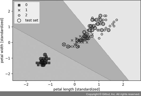
▲ 그림 3-6 사이킷런의 로지스틱 회귀 모델이 만든 결정 경계