다음은 최적화 결과를 차트로 그리기 위한 코드다. 코드는 n개의 종목으로 다양한 투자 비중을 조합해 구성한 30,000개의 포트폴리오를 만든다. 투자 비중은 랜덤하게 정해지며, 그 합계는 1.0(100%)이다. 또한, 수익률, 위험을 계산하고 수익률, 위험, 투자 비중을 리스트에 담는다.
그리고 matplotlib를 이용해 여러 가지 효과를 준 분산형 차트로 그린 것이다.
p_returns = [ ]
p_volatility = [ ]
p_weights = [ ]

n_assets = len( tickers )
n_ports = 30000

for s in range( n_ports ):
    wgt = np.random.random( n_assets )
    wgt /= np.sum( wgt )
    ret = np.dot( wgt, ret_annual )
    vol = np.sqrt( np.dot( wgt.T, np.dot(cov_annual, wgt ) ) )
    p_returns.append( ret )
    p_volatility.append( vol )
    p_weights.append( wgt )

rets = np.sum( ret_daily.mean( ) * res[ 'x' ] ) * 250
vol = np.sqrt( res[ 'x' ].T @ covmat @ res[ 'x' ] )
p_volatility = np.array( p_volatility )
p_returns = np.array( p_returns )

colors = p_returns/p_volatility
plt.style.use( 'seaborn' )
plt.scatter( p_volatility, p_returns, c=colors, marker='o', cmap=mpl.cm.jet )
plt.scatter( vol, rets, marker="*", s=500, alpha=1.0 )
plt.xlabel( 'Volatility (Std. Deviation)' )
plt.ylabel( 'Expected Returns' )
plt.title( 'Efficient Frontier' )
plt.show( )
결과
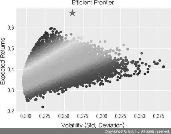
▲ 그림 4-21 샤프비율 최적화 결과